The Gradient descent algorithm we saw in an earlier post just gives you an idea of how gradient descent works. We’ve seen that
$$W \leftarrow W - \alpha E’(W)\\
$$
This is just a rough formula to get you started. In practice what $E’(W)$ is calculating is the average of all the gradients due to every point in your training data. This is known as Vanilla Gradient Descent or Batch Gradient Descent. Large datasets with millions of instances are easily available nowadays. This presents a challenge to the vanilla gradient descent. The weights are updated after calculating the average of all the data points available, which significantly increases training time.
Let’s see some optimizations to keep these under control.
Stochastic Gradient Descent
The trivial solution to overcome this problem is that you update the weights for every instance. This is known as Stochastic Gradient Descent. This reduces our training time in terms of updating the weights. But in practice, this method approaches the minima rather slowly. This is due to the fact that each of the instances is biased and generally doesn’t point in the direction of the global minima.
Mini Batch Gradient Descent
To gain the advantages of both of these techniques, we can achieve a trade-off by calculating the average of some instances. This is called the mini batch gradient descent. Mini Batch refers to the number of instances we consider to compute the gradient. In practice, it varies from 8 to 256, with more larger numbers rarely used. The illustration below summarizes all the variants of gradient descent we’ve seen so far.
Adaptive Learning Rate
With gradient descent we can be sure that we’ll be better off on each of the iterations of training. But this does come at a cost. While during initial stages the loss can drop down dramatically and then the drop in loss becomes so small that you’ll be on the verge of giving up on your whole network. This may be due to the fact that there are many places where the gradient is stuck between valleys or the movement towards the minima is so small. Also there are surfaces which curve more steeply along one dimension and less along other. These are called ravines. Stochastic Gradient Descent oscillates along the slopes of the ravine and makes little progress towards the minimum.
To mitigate these problems to a certain extent, we give gradient descent some memory of its previous steps, so as to control the oscillations and take a more bold step towards the minima. This is the general idea of momentum. It can also adjust the learning rate according to the previous progress achieved by the gradient descent.
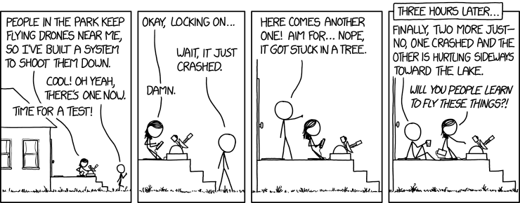
We’ll see more details about momentum and will start a mini-series on the gradient descent optimization algorithms. Till then soak all the things we’ve seen so far and enjoy the comic.
